
Created: Sat 11 July 2026 / Last updated: Wed 29 July 2026
This is the author's version of the preprint published on ChemRxiv, doi:10.26434/chemrxiv.15006045/v1. The models it describes power the free property predictor at chemeo.com/predict.
Loïc d'Anterroches, Céondo GmbH, loic@ceondo.com.
Abstract
A message-passing neural network is a learned group-contribution method only if its readout carries molecular size, which the framework-default mean readout discards. We train directed message-passing neural networks (D-MPNN, Chemprop v2) on experimental thermophysical data from the Cheméo database, one model per property, as a general-purpose graph-based alternative to the Joback group-contribution method [14], strongest in the regime where Joback degrades: Joback was fitted on small molecules and, as we show here head-to-head, degrades steadily as molecules grow; those larger molecules are a minority of the corpus (a quarter to a third of a typical set has eleven or more heavy atoms, though the spread is wide, from 11% for the small Gibbs-energy set to 56% for melting point), but they are exactly the regime where a group-contribution method has no good alternative. The contribution is not that sum pooling beats mean pooling, a fact already established in the graph-learning literature [18,19]; it is a property-by-property diagnosis on experimental thermophysical data of how the default silently fails, a reusable release discipline, and a family of released models measured against Joback, a simple descriptor baseline, and external data. The mean readout is size-invariant: it returns the average per-atom contribution, so a molecule and its dimer map to nearly the same vector, and every property that tracks molecular size collapsed toward the training mean; six properties, among them the critical constants and the Gibbs energy of formation, landed at test R² near zero, and a gradient-boosted tree on plain RDKit descriptors beat the graph network on all six. Replacing the mean with a sum-aware pooling (sum and max concatenated) makes the molecule embedding scale with atom count, and the message passing then learns the higher-order structural corrections that Marrero and Gani add to a classical scheme by hand as second- and third-order groups [15]. The distinction we keep is between a graph-extensive readout (a property of the network) and a thermodynamically extensive target: the sum is needed outright for extensive targets such as critical volume and the formation enthalpies, while intensive targets that rise along homologous series, such as the boiling and critical temperatures, benefit because molecular size is a strong predictor of them, not because they are extensive. Nine of sixteen properties are released under a two-part criterion: a statistical bar (mean out-of-sample R² above 0.70 with a train-test gap of at most 0.20 under repeated scaffold cross-validation, or state-of-the-art accuracy on a shared external benchmark) and a veto, that the incumbent Joback must not significantly out-predict the model in its tested domain; we lead with mean absolute error, since a small scaffold test set makes R² noisy: normal boiling point (MAE 13.5 K, RMSE 30 K, 3.5% average relative error), melting point (MAE 30.8 K), critical volume and critical temperature, enthalpies of formation and vaporisation, ionisation energy, aqueous solubility and the acentric factor, each reported against Joback, the published state of the art, and the experimental reproducibility floor of the property. Against Joback on identical held-out folds the graph model significantly wins on five of the nine comparable properties (boiling-point MAE 13.5 vs 26.3 K, formation enthalpy 35.5 vs 70.9 kJ/mol), ties two, and its error grows far more slowly with molecular size than Joback's, which grows several-fold; it also covers the compounds Joback cannot fragment at all, a few percent of a typical set and up to about 12% for some properties, at undiminished accuracy on the ordinary organics among them; the two properties Joback still out-predicts, Gibbs energy of formation and critical pressure, are exactly the two the veto holds back as beta, with Joback served in their place. We release them as the Cheméo Relay family, one model per property.
Keywords: message-passing neural network, group contribution, thermophysical properties, critical properties, aqueous solubility, machine learning.
1. Introduction
Cheméo already offers property predictions through its API, computed with the Joback group-contribution method [14]. Group contribution is the workhorse of thermophysical estimation: a property is the sum of contributions from the functional groups in the molecule. It is fast, transparent, and good on the small, well-behaved molecules it was fit on. It also has a known weakness, and it is a weakness of the summation itself. The larger and more complex the molecule, the more groups are summed, the more the per-group errors accumulate, and the more the first-order groups miss the longer-range structure that a big molecule actually has. The Marrero-Gani method answers this by adding second- and third-order groups, larger fragments that act as corrections on top of the first-order sum [15]. Those higher-order groups work, but someone has to define and fit them by hand.
We wanted the correction to be learned rather than curated. A message-passing graph network is the natural tool: it learns an embedding per atom from the atom's neighbourhood, then pools the atoms into a molecule vector. If the pooling is a sum, the model is doing what a group-contribution method does, summing local contributions, except that the contributions and their higher-order corrections are learned end to end instead of tabulated. That is the model we set out to build: a graph-based, general-purpose replacement for Joback that holds up on the large molecules where Joback breaks, trained on a broad experimental corpus.
The paper keeps the diagnostic path visible, not only the final numbers, because mean pooling is the framework default and the failure is silent: training converges, the loss curves look normal, and the model predicts the average. The same defect will catch anyone training graph models on any property that varies with molecular size, extensive or merely size-correlated, in any framework.
The corpus consists primarily of fluid-phase thermophysical properties: boiling and melting points, the critical constants, the formation and phase-change enthalpies, the acentric factor, aqueous solubility. Three of the sixteen (ionisation energy, electron affinity, dipole moment) are electronic rather than fluid-phase; we keep them, and mark them as such, because they are a useful out-of-domain check that the readout finding is a general property of the network and not a quirk of thermophysical targets. The released family and every headline claim rest on the fluid-phase properties; the electronic ones are supporting evidence, and a reader interested only in the thermophysical core can read the electronic-property rows as a generality control.
2. The model
We use the Chemprop v2 directed message-passing neural network [1,2]. It reads a molecule as a graph, atoms are nodes and bonds are edges, and turns it into one property value in four stages (Figure 1).
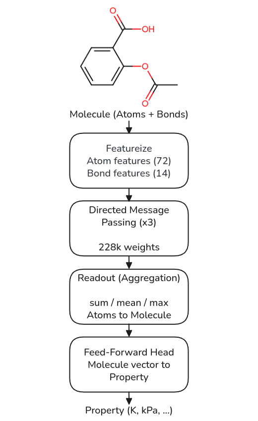
Figure 1. The four stages of the D-MPNN, with the number of trainable weights at each stage.
The first stage is featurisation, and it has no learned weights. Each atom is described by a fixed vector (atomic number, degree, formal charge, chiral tag, hydrogen count, hybridization, aromaticity and mass, 72 numbers) and each bond by a smaller one (bond type, conjugation, ring membership and stereochemistry, 14 numbers).
The second stage is the message passing, and it is where almost all the weights live. A hidden state sits on each directed bond and is updated for a few steps, three in our models, from the other bond messages arriving at its source atom. The word "directed" matters: a bond does not send its message straight back the way it came, which keeps information flowing outward instead of echoing. One shared weight matrix does every update at every step, so the network learns a single local function and applies it everywhere in the molecule. A shared local update, reused for every atom, is the learned counterpart of a group contribution; Section 5 builds on this. After the passes, the bond messages are gathered onto their atoms, giving one learned vector per atom.
The third stage is the readout, which pools the per-atom vectors into one molecule vector by summing, averaging or taking the maximum. It has no weights of its own, and it is the choice everything below depends on.
The fourth stage is a small feed-forward head that maps the molecule vector to the property, in physical units, with the target scaler fit on the training split only.
The weight budget is modest. With a mean readout the model has about 318,000 trainable weights: roughly 228,000 in the shared message passing, about 91,000 in the head, and none in the readout. A richer readout does not touch the message passing at all; it only widens the head, by about 90,000 weights for sum+max and 180,000 for mean+sum+max. So when we compare readouts later, it is the same graph encoder with a slightly larger or smaller final layer, not a different network.
We chose Chemprop because it is a maintained implementation with sensible defaults, but nothing in this work depends on it. Appendix A gives the complete recipe: the exact atom and bond features, the message-passing equations, every hyperparameter, the training schedule, the descriptor set and its scaling, and the diagnostic procedures. Anyone can reproduce this in PyTorch Geometric, DGL, or from scratch, without installing this package.
3. Data
Experimental values come from the Cheméo API [17], with all computed values (group-contribution or quantum estimates) excluded, so the training targets are measurements and not another method's predictions. This is the first line of defence against a legitimate circularity concern, that a model advertised as replacing group contribution might be trained on group-contribution numbers. It is not a complete guarantee, and the critical constants are the main concern: many larger molecules thermally decompose before reaching their critical point, so a tabulated "experimental" $T_c$, $P_c$ or $V_c$ is frequently a correlation-derived estimate rather than a direct measurement, produced upstream of Cheméo and beyond our filtering. This is one reason we treat the critical constants with caution (Section 8.1). Cheméo's SMILES is stereo-stripped, so structures are parsed from the InChI first (it keeps the stereo layers), falling back to SMILES; records with no heavy atom (bare elements) are dropped. When a compound has several measurements they are collapsed to the median, and the pipeline logs any compound whose measurements disagree by more than a set fraction of the median, so gross inconsistencies surface rather than being averaged away silently; each row keeps a measurement count and a min-to-max spread. The redundancy is uneven: the large sets are well backed (about half of the boiling-point, solubility, ionisation-energy and vaporisation compounds carry more than one measurement), while several of the small, held-back or borderline properties (critical compressibility, acentric factor, Gibbs energy, dipole moment) are single-source per compound, so their scatter cannot be checked internally. Per-property counts, the multi-measurement fraction and the coarse plausibility-range filter applied to drop corrupt records are tabulated in Appendix A.6. Values are then split by Bemis-Murcko scaffold into 0.8 / 0.1 / 0.1 train / validation / test. The scaffold split matters: it forces the test set to contain whole scaffold families the model never saw, so the numbers reflect generalisation and not memorisation.
4. Failure of the mean readout on size-dependent properties
The first pass trained one D-MPNN per property with the Chemprop defaults, which include mean aggregation. Several properties trained well. Six did not: critical temperature, critical pressure, critical volume, critical compressibility, Gibbs energy of formation and enthalpy of fusion all landed at R² near zero, no better than predicting the training mean. The published state of the art for some of these is R² above 0.9, so R² near zero is a red flag for a data or pipeline problem, not a model-capacity limit.
We ran the cheapest useful diagnostic first: a gradient-boosted decision-tree regressor (a GBM) on a dozen plain RDKit [16] descriptors, on the same split. If a simple tree model predicts a property well from basic descriptors but the graph network scores near zero, the data is learnable and the bug is in our neural-network pipeline.
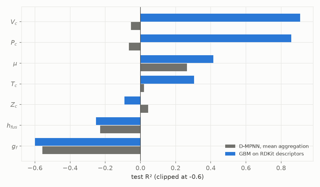
Figure 2. Test R² of a gradient-boosted tree on RDKit descriptors and of the mean-aggregation D-MPNN, for the six low-R² properties, on the same scaffold split.
The tree model outperforms the graph network on all six properties (Figure 2), most sharply on critical volume: R² 0.91 for the GBM against a negative R² for the graph network. The data is learnable; the defect is in our neural pipeline.
The GBM has molecular weight and heavy-atom count as inputs. The graph network does not, in any usable form, because mean aggregation averages the per-atom embeddings and throws molecular size away. Two molecules with the same average atom but different sizes map to the same vector. For a property that scales with size, like a critical volume or a formation energy, the readout cannot represent the thing that varies, so the best the model can do is regress toward the mean.
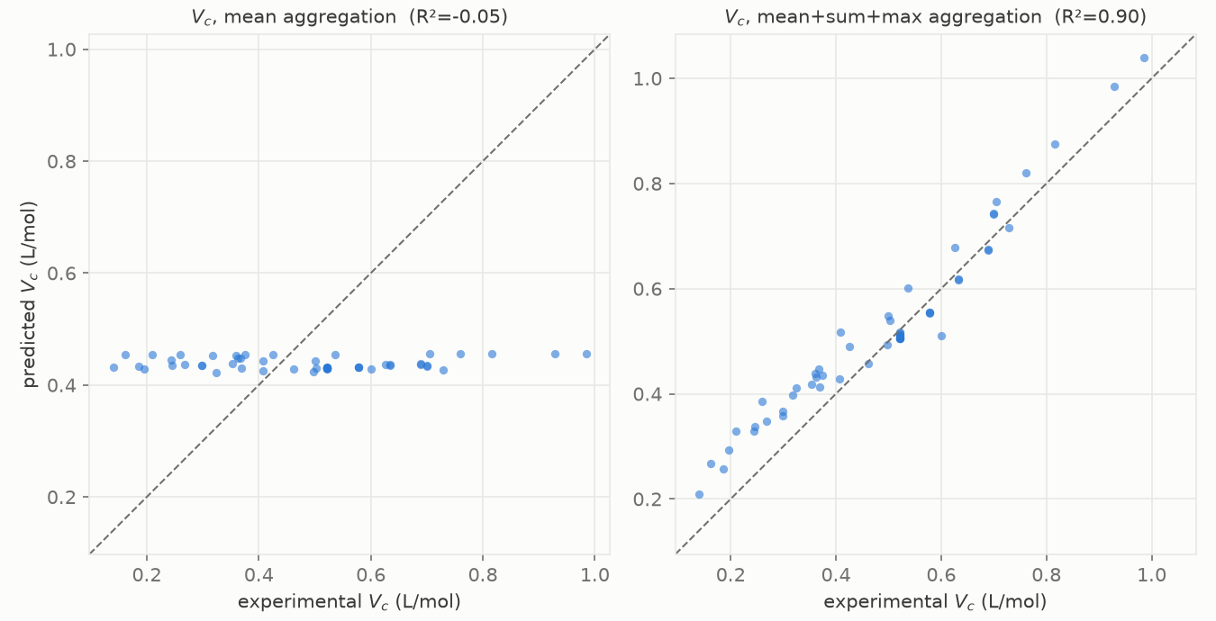
Figure 3. Predicted against experimental critical volume, for the mean readout (left) and the mean+sum+max readout (right), same network and scaffold split.
On the left, with mean aggregation, the predictions form a flat horizontal line (Figure 3): whatever the true critical volume, the model returns about 0.44 L/mol. That is the mean collapse. On the right, with a size-aware readout, the same network on the same split lands on the diagonal.
5. The readout must carry molecular size
The readout pools the per-atom embeddings into one molecule vector. Chemprop provides mean, sum and norm; sum and its relatives keep molecular size, mean does not. Two more pooling operations are a few lines each, because the same scatter call that does mean and sum also does max and min: max keeps the single most extreme atom per feature, which is the signal a lone functional group carries and the average washes out.
We compared four readouts across all properties, changing only the readout and nothing else, with best-validation weights restored so the comparison is not polluted by where early stopping happens to stop.
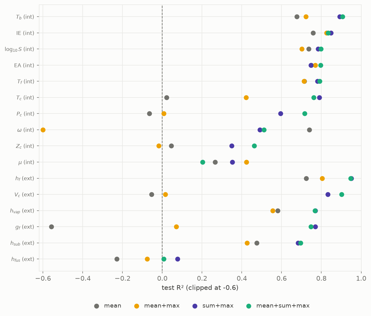
Figure 4. Influence of aggregation form on R² at constant message-passing layer. Each row is one property, labelled by whether the target is thermodynamically extensive (ext, scales with amount of substance: critical volume, the formation energies, the enthalpies) or intensive (int, does not: the temperatures, pressures, acentric factor, electronic properties). The four points per row are the readouts shown in the key. Test R², clipped at -0.6.
Two claims have to be kept apart, and for a thermodynamics readership the distinction matters. The first is about the network: a sum readout makes the molecule embedding graph-extensive, meaning it scales with the number of atoms, because it is a sum of per-atom contributions. That is exactly what a group-contribution method computes, and it is a property of the pooling, not of any target. The second is about the targets: some are thermodynamically extensive and some are not. Critical volume (molar), the formation energies and the vaporisation enthalpy grow with molecular size, so a size-carrying readout is not optional for them; the mean, which divides the summed contributions by atom count and so is size-invariant, cannot represent what varies, and the model regresses to the mean. The boiling and critical temperatures, the critical pressure and the acentric factor are intensive: they do not scale with amount of substance. They still improve with a sum readout, but for a different reason, because along a homologous series they rise smoothly with molecular size, so size is a strong predictor even though the property is not extensive. The mean discards that predictor; the sum keeps it. The two must not be conflated: calling an intensive property "extensive" because a size-aware readout helps it is a category error. The readout is graph-extensive; the target may or may not be.
Where the neural and the classical methods meet is the corrections. Methods such as Marrero-Gani add second- and third-order groups by hand to fix the first-order sum on larger molecules [15]; the message passing learns the equivalent correction by making each atom's contribution a function of its neighbourhood, so the higher-order structure is already inside the summed contributions.
That sum pooling is more expressive than mean pooling is not a new claim in graph learning, and we do not present it as one. Xu et al. [18] proved that a sum aggregator is strictly more discriminative than mean or max for distinguishing multiset neighbourhoods, and Corso et al. [19] introduced Principal Neighbourhood Aggregation, concatenating several aggregators (mean, sum, max, min, with degree scalers) for exactly the reason we concatenate sum and max here. Our sum+max readout is a two-channel special case of that recipe. What is new is not the pooling but the demonstration: a property-by-property account, on experimental thermophysical data, of how the framework default silently collapses on the properties a thermodynamicist actually wants, with the group-contribution reading of why and a release discipline built around it.
Two consequences for the readout choice follow from Figure 4. First, sum+max beats mean+max, clearly on the extensive properties: on critical volume, mean+max reaches R² 0.02 while sum+max reaches 0.83 on the frozen seed-42 split. The sum channel, not the max channel, is what carries size. Second, sum+max at two thirds of the width rivals the full mean+sum+max, so it is the lean default when the target tracks size. A mean+max readout can score below the plain mean, so a max channel does not substitute for the missing sum channel.
Because Section 6 shows a single scaffold split is noisy on the smaller sets, the ranking in Figure 4 could in principle be a split artifact there, so we repeat the four-way comparison over three independent scaffold splits (seeds 42-44) and report the spread (test R², mean ± sd):
| property | n | mean | mean+max | sum+max | mean+sum+max |
|---|---|---|---|---|---|
| IE | 5302 | 0.80±0.02 | 0.80±0.02 | 0.81±0.02 | 0.82±0.01 |
| $T_b$ | 4948 | 0.68±0.05 | 0.71±0.01 | 0.72±0.03 | 0.73±0.03 |
| $T_f$ | 4433 | 0.15±0.34 | 0.45±0.38 | 0.48±0.32 | 0.44±0.45 |
| $\Delta H_{vap}$ | 2496 | 0.30±0.08 | 0.25±0.12 | 0.42±0.07 | 0.45±0.07 |
| $\Delta H_f$ | 2337 | 0.82±0.03 | 0.82±0.04 | 0.98±0.00 | 0.98±0.01 |
| $\log_{10}S$ | 2104 | 0.30±0.08 | 0.53±0.01 | 0.72±0.02 | 0.72±0.01 |
| $\Delta H_{sub}$ | 1343 | 0.06±0.15 | 0.19±0.15 | 0.47±0.05 | 0.51±0.05 |
| $T_c$ | 1054 | 0.82±0.03 | 0.80±0.02 | 0.84±0.01 | 0.86±0.01 |
| $P_c$ | 917 | 0.52±0.08 | 0.62±0.02 | 0.60±0.06 | 0.56±0.04 |
| EA | 637 | 0.50±0.12 | 0.44±0.05 | 0.54±0.04 | 0.40±0.03 |
| $\omega$ | 599 | 0.76±0.01 | 0.76±0.03 | 0.83±0.01 | 0.83±0.02 |
| $V_c$ | 549 | 0.86±0.03 | 0.92±0.01 | 0.96±0.00 | 0.96±0.00 |
| $\Delta H_{fus}$ | 525 | -0.14±0.03 | -0.20±0.05 | -0.18±0.04 | -0.21±0.05 |
| $Z_c$ | 511 | 0.21±0.08 | 0.13±0.08 | 0.36±0.06 | 0.24±0.13 |
| $\Delta G_f$ | 332 | 0.65±0.18 | 0.53±0.07 | 0.88±0.05 | 0.84±0.02 |
| $\mu$ | 301 | 0.54±0.17 | 0.57±0.07 | 0.66±0.09 | 0.45±0.22 |
Table 1. Test R² over three scaffold splits, four readouts, graph-only. Bold is the best readout per row. This also gives each property a seed-to-seed R² spread (the small-set-variance issue of Section 6): tight on the large sets ($\Delta H_f$, $V_c$, IE ± ≤ 0.02), wide on the smallest and hardest ($T_f$ ± 0.3), as expected.
A size-carrying readout (sum+max or mean+sum+max) is the best of the four on fourteen of the sixteen properties, and sum+max beats mean+max on the same fourteen, so the ranking is not a single-split artifact: the sum channel carries size across seeds. The two exceptions are minor. On enthalpy of fusion every readout is near or below zero, so there is no size signal to carry (it is a crystal-packing property, Section 8.1). On critical pressure mean+max (0.62±0.02) edges sum+max (0.60±0.06) within overlapping error bars, a tie rather than a reversal. The spread also makes Section 6's point concrete from the other direction: the same model and readout swing by ±0.3 R² on melting point across seeds, so no single split should be trusted on the small, hard sets.
The same size-blindness explains an earlier result we had misread. Concatenating whole-molecule descriptors (molecular weight, shape, H-bonding) had brought boiling-point MAE down from 34.6 K to about 16 K, which we first credited to the descriptors; in fact they helped only by supplying the molecular size that mean aggregation discards, and a size-aware readout reaches the same accuracy on its own, without computing any descriptors.
5.1 The readout versus a per-heavy-atom target
There is a cheaper-looking way to give a mean-readout network the missing size: divide the extensive target by the heavy-atom count before training and multiply back afterwards. This is the classical group-contribution normalisation, it needs no architecture change, and it is fair to ask whether it makes the readout change unnecessary. We tested it directly on the five extensive properties, on the frozen seed-42 split, comparing four configurations that differ only in readout and target (test R²):
| property | A: mean, identity | B: mean, per-heavy-atom | C: sum+max, identity | D: sum+max, per-atom |
|---|---|---|---|---|
| $V_c$ | -0.05 | 0.99 | 0.83 | 0.95 |
| $\Delta G_f$ | -0.56 | 0.85 | 0.77 | 0.46 |
| $\Delta H_f$ | 0.74 | 0.91 | 0.94 | 0.94 |
| $\Delta H_{vap}$ | 0.57 | 0.81 | 0.77 | 0.80 |
| $\Delta H_{fus}$ | -0.23 | -0.97 | 0.08 | -0.95 |
Table 2. Test R² on the frozen seed-42 split; A is the collapsed baseline. Bold marks the best of the four per row.
The per-heavy-atom target (B) is a real and sometimes stronger alternative: on critical volume and Gibbs energy it beats the sum readout (C), because those targets are cleanly extensive and dividing by size turns them into a well-behaved intensive quantity. But it has two failure modes the readout does not. It is fragile: on enthalpy of fusion the per-atom value is small and noisy and the multiply-back step amplifies the error on large molecules, so config B collapses to R² -0.97, worse than doing nothing (A). And it is property-specific: it requires knowing in advance that the target is extensive and would actively harm an intensive but size-correlated target such as the boiling or critical temperature, which must not be divided by atom count. The sum readout (C) needs neither assumption: it is positive on all five properties, never catastrophic, and it is the same single architectural change for extensive and intensive targets alike. Stacking both (D) is not reliably better than either alone. We therefore use the readout as the primary lever and leave the target in physical units, while noting that for a known-extensive property a per-heavy-atom target is a legitimate, occasionally better, alternative.
6. Dataset size, overfitting and seed variance
Making the readout wider adds weights to the feed-forward head, so overfitting is a real concern on the smaller property sets, where the 10% validation split is only a few dozen molecules and early stopping rides on a noisy signal. We measured it directly by the train-minus-test R² gap for every property.
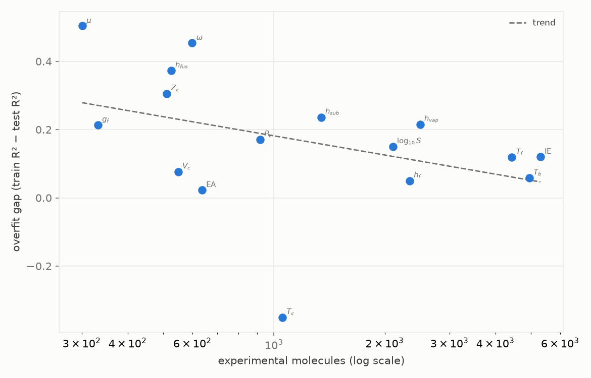
Figure 5. Train-minus-test R² gap against the number of experimental molecules per property (mean+sum+max model, log scale). The line is a least-squares trend.
The trend is plain (Figure 5): more data, smaller gap; less data, wider gap. It is a trend, not a cutoff. It says the small-data models are less stable, not that they cannot be built: some sub-thousand sets still generalise cleanly out-of-sample (Section 8). The lesson is caution: with little data the overfitting risk is higher, so the evaluation has to work harder to tell a real result from a lucky one.
The gap is one face of small data; the seed is the other. We repeated every property under five seeds, each drawing its own scaffold split and running its own training, and looked at the spread of test R² (Figure 6).
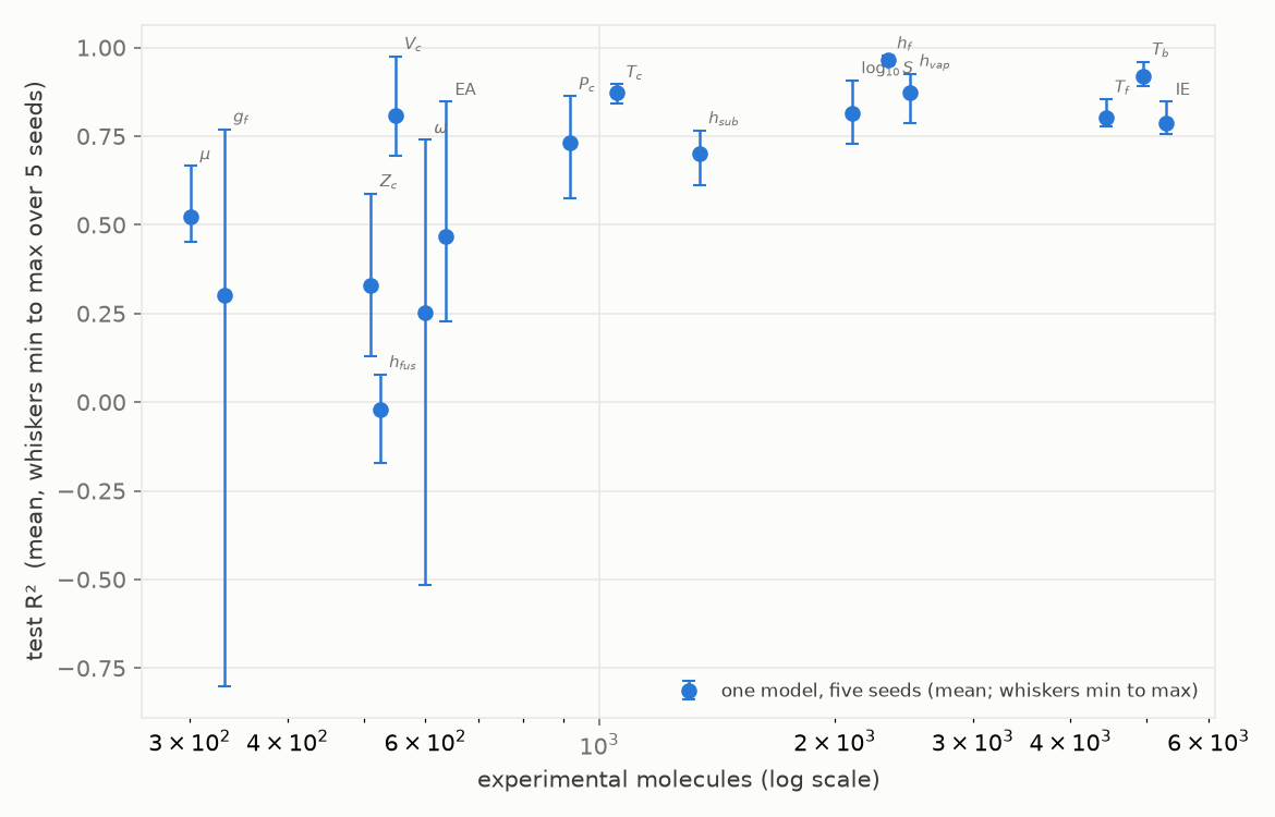
Figure 6. Test R² per property against the number of experimental molecules (log scale). Point is the mean over five seeds, whiskers span the minimum to the maximum; each seed draws its own balanced Bemis-Murcko scaffold split.
The pattern is clear. Above about a thousand molecules the five seeds agree within a few R² points: the number does not depend on which molecules happened to fall in the test set. Below it the spread widens sharply: the acentric factor swings from R² -0.52 to 0.74 on the seed alone, Gibbs energy of formation from -0.80 to 0.77. A different seed on the same model and data can therefore report almost any value, and selecting the best seed amounts to selecting the top of that spread and calling it the model. The implication for small data is not that the models cannot be built, but that a single favourable split is not evidence: the evaluation has to be robust to the choice of split.
This is why the evaluation cannot rest on a single split. It has to be scaffold-aware, whole scaffold families held out so the test measures generalisation and not memorisation, and it has to test every compound rather than a lucky ten percent. On small, unbalanced data the folds themselves are delicate: about half of these sets are acyclic, and a naive scheme that pools every acyclic molecule into one group leaves that fold enormous and the rest starved, which breaks the very method meant to guard against the instability. Section 9 builds the evaluation that handles this: repeated scaffold cross-validation, with the acyclic molecules spread across the folds.
7. Descriptor augmentation: 2D is roughly neutral, a single-conformer 3D set adds noise
With the readout fixed per property, we measured what the descriptors still add. For each property we trained three models that differ only in the extra inputs: the graph alone, the graph plus 15 two-dimensional descriptors (no conformer), and the graph plus all 23 descriptors, the extra 8 being shape and dipole terms that need a 3D conformer.
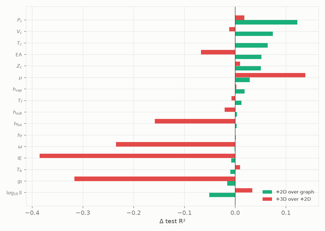
Figure 7. Change in test R² from adding descriptors to each property's best readout: 2D descriptors over graph-only, and 3D-conformer descriptors over 2D.
Adding the 2D descriptors moves the average test R² by only about +0.02 (Figure 7), which is inside the seed-to-seed spread documented in Section 6 and so not distinguishable from zero on average; the 2D set is roughly neutral overall while clearly helping a handful of properties (critical pressure, critical volume, critical temperature, electron affinity), which is why we keep it only where it earns at least +0.01 R² and use the graph alone everywhere else. Adding the 3D descriptors makes it worse on average, about -0.06 R², with large losses on ionisation energy, Gibbs energy and the acentric factor. The 8 shape and dipole terms are computed from a single ETKDGv3 conformer with a fixed random seed, MMFF-optimised: one conformer is a noisy sample of the real conformational ensemble, so these features add noise more than signal, and on a few hundred to a few thousand points that noise overfits. This limitation is specific to the single-conformer descriptor set, not to 3D information in general; a proper conformer-ensemble average could well behave differently and we have not tested it.
On this data the 3D-conformer descriptors are net-negative, so we do not use them: each property's best model is the graph alone, or the graph with the conformer-free 2D descriptors where those add at least a small lift.
8. The released models
The release rule has two parts, and both are needed to make the list track practical usefulness rather than a mechanical cut. The statistical part is the bar under repeated scaffold cross-validation (Section 9): mean out-of-sample R² above 0.70 with a train-test gap of at most 0.20, or, for a property the scaffold CV is demonstrably too hard on, validation on a shared external benchmark at the state of the art (Section 8.1). The second part is a veto: whatever the statistics, we do not release a model that the incumbent it is meant to replace, Joback, significantly out-predicts in the domain we can test (significance by the paired bootstrap of Section 8.2). A property is released, in short, when it is the best trustworthy predictor we can offer for it. The veto changes the list in both directions relative to the bar alone: critical temperature sits below the CV bar (R² 0.657) but is externally validated at the state of the art and significantly beats Joback, so it is released; Gibbs energy of formation clears the CV bar (R² 0.840) but Joback significantly out-predicts it, so it is held as beta. We prefer the graph-only model unless the 2D descriptors add at least a little. Cross-validation replaced the single five-seed split as the statistical gate once we found that split unreliable in both directions on the smaller sets: it flattered two models and condemned two others (Section 9). The numbers below are out-of-sample under repeated scaffold 10-fold cross-validation (three repeats), every compound held out exactly once. We lead with mean absolute error, in the property's own units, because on these small scaffold test sets R² rides on a noisy variance denominator; RMSE is given alongside, and the group-contribution (Joback) and gradient-boosted-tree baselines on the same folds are in Section 8.2. One caveat on the R² column, which the next section returns to: it is pooled across all folds, so its denominator is the variance of the whole dataset, not of a single 10% test slice. That makes it larger, and not directly comparable to the single-split R² quoted in the diagnostic sections. Critical volume is the clearest case: R² 0.83 on the frozen seed-42 split in Section 5 (where the matched GBM scored 0.91) and R² 0.988 pooled here are the same model measured two ways, not a contradiction; the single-split number is the one to compare against the GBM, the pooled number the one to compare across properties. Nine of the sixteen properties are released.
| Property | Symbol | Unit | model | n | CV MAE | CV RMSE | CV R² | AARD |
|---|---|---|---|---|---|---|---|---|
| Enthalpy of formation (gas) | $\Delta H_f$ | kJ/mol | graph | 2337 | 35.5 | 64.5 | 0.974 | n/a |
| Normal boiling point | $T_b$ | K | graph | 4948 | 13.5 | 30.2 | 0.879 | 3.5% |
| Enthalpy of vaporisation | $\Delta H_{vap}$ | kJ/mol | +2D | 2496 | 3.69 | 6.75 | 0.949 | 6.8% |
| Aqueous solubility | $\log_{10}S$ | log₁₀(mol/L) | graph | 2104 | 0.560 | 0.771 | 0.877 | n/a |
| Critical volume | $V_c$ | L/mol | +2D | 549 | 0.0156 | 0.0242 | 0.988 | 5.3% |
| Normal melting point | $T_f$ | K | +2D | 4433 | 30.8 | 56.3 | 0.744 | 10.2% |
| Ionisation energy | IE | eV | graph | 5302 | 0.344 | 0.608 | 0.795 | 4.0% |
| Critical temperature | $T_c$ | K | +2D | 1054 | 33.1 | 84.8 | 0.657* | 6.8% |
| Acentric factor | $\omega$ | (dimensionless) | graph | 599 | 0.0512 | 0.0795 | 0.781 | n/a |
Table 3. The nine released models and their out-of-sample error under repeated scaffold 10-fold cross-validation (three repeats, seeds 42-44). MAE and RMSE are in each property's own units, n is the number of experimental molecules, and AARD is the average absolute relative deviation. () Critical temperature is released under the external-benchmark arm of the rule (Section 8.1).*
MAE, RMSE and R² are out-of-sample under repeated scaffold 10-fold cross-validation (three repeats, seeds 42-44), averaged over repeats; n is the number of experimental molecules for the property. They are the numbers from one canonical run, the head-to-head of Section 8.2, so the released models and their Joback/GBM baselines are read from a single evaluation. An earlier, independent cross-validation run gives the same values up to small run-to-run variation across the CV repeats (for instance boiling point 13.5 here versus 13.8 there); that is seed- and initialisation-level variability, not a metric discrepancy, and we quote the head-to-head run everywhere to keep one basis. (*) Critical temperature is the one release below the CV bar: it enters under the external-benchmark arm of the rule, R² 0.916 on the held-out CRC set (Section 8.1), and it significantly beats Joback (Section 8.2). We show its conservative scaffold-CV number in this table, not only the flattering external one, because Section 9 argues the scaffold number is the harder test: for $T_c$ the CV population is small and unusually diverse, so 0.657 is the pessimistic bound and 0.916 the benchmark the field reports on. AARD (average absolute relative deviation, $\langle|\hat y - y|/|y|\rangle$, from the per-repeat out-of-sample predictions) is quoted only for the properties with a natural zero and no sign change, where a relative error is meaningful (it is not for the formation energies, solubility or acentric factor). For the temperatures the reference is absolute (0 K): the 3.5% for $T_b$ is relative to the absolute boiling temperature, not a Celsius scale. The boiling-point RMSE/MAE ratio is high (30.2 / 13.5 ≈ 2.2), which signals a heavy tail of a few large misses rather than a uniformly larger error. The tail is not the large-molecule tail: the twenty worst-predicted compounds average 9.1 heavy atoms, essentially the dataset mean (9.3), and error correlates negligibly with size (r ≈ 0.06), so the outliers are scattered across the size range (unusual chemistries and hard individual measurements) rather than concentrated in the large-molecule tail. Six models are graph-only, three use the 2D descriptors, none uses 3D.
Two properties clear or approach the statistical bar yet are held as beta, both under the Joback veto, and for both Cheméo continues to serve the Joback estimate as the recommended value alongside the beta graph model. Gibbs energy of formation clears the CV bar (R² 0.840) but Joback significantly out-predicts it (MAE 22.4 vs 42.2 kJ/mol, bootstrap CI on the difference $[+9.4, +24.3]$, and Joback wins every size bin); it has no external check, and its size-extrapolation case is undemonstrated on its own corpus (the large-molecule bins hold 20 and 15 compounds). It returns to full release if more large-molecule Gibbs-energy data shifts the balance. Critical pressure fails the CV bar (R² 0.585) and the veto (Joback 300 vs 487 kPa, CI $[+37, +90]$), and it fails the size-extrapolation story too: Joback's $P_c$ error does not grow with molecular size (470 kPa in the smallest bin, 164 in the largest), so there is no regime on this corpus where the graph model is the better $P_c$ predictor. Two data limits cloud the target itself and are the next collection priority: the set is small (n = 917) and many tabulated critical pressures are themselves group-contribution estimates, contaminating both the training labels and the external CRC labels.
The five we do not release at all are enthalpy of sublimation, electron affinity, dipole moment, critical compressibility and enthalpy of fusion (all sixteen properties, released, beta and held, are tabulated with their CV numbers in Appendix A.9). Enthalpy of sublimation is the closest miss: its mean R² is 0.70, right on the bar, but its overfit gap is just past the 0.20 line and it has no external set to enter by, so it waits for more data.
Two properties were nearly lost to the evaluation itself, and how they were recovered matters for the method. Gibbs energy of formation and the acentric factor were near-zero under a single seed (mean R² 0.30 and 0.25 over ranges of order a full R² unit) and would have been dropped for seed variance. Cross-validation shows the instability was small-test-set noise, not model instability: each is stable across fold partitions (repeat sd about 0.01), clears the gap criterion, collapses to R² near zero under a label-shuffle control (so it is learning structure, not memorising), holds under a similarity-cluster leakage control, and scores R² about 0.80 on the ring-containing compounds that make up the single-split test population. Both are therefore legitimate models rather than seed-variance artifacts; the acentric factor is released, and Gibbs energy goes to beta not because its statistics fail but because the veto bites, Joback still predicts it better (Section 8.2). The single 10% scaffold split is unreliable in both directions on small sets: it flattered the critical constants and it condemned these two.
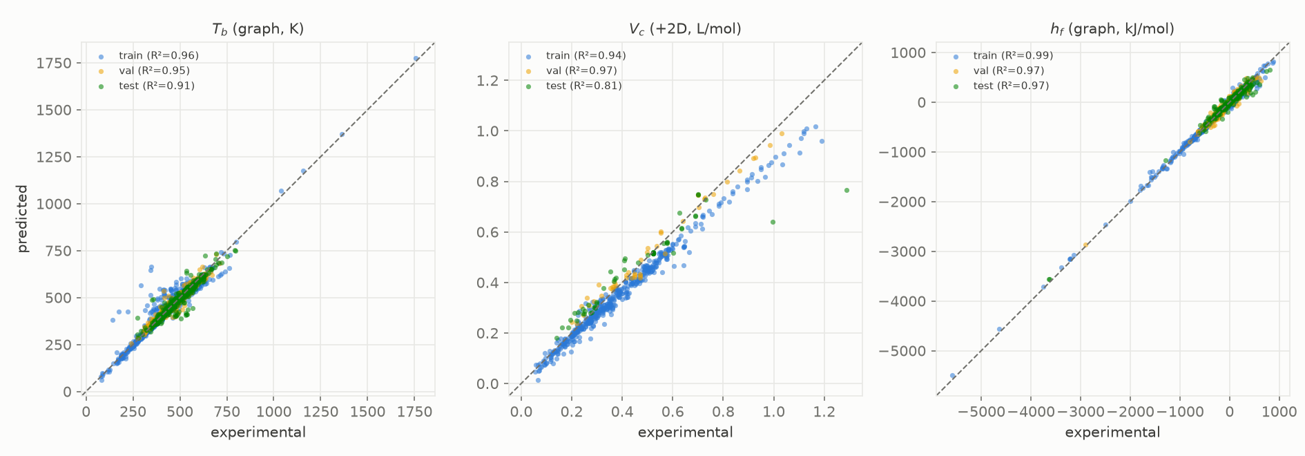
Figure 8. Predicted against experimental for three released models ($T_b$, $V_c$, $\Delta H_f$), coloured by data split, all molecules.
Two of these numbers are much better than in our own first pass (Figure 8). Enthalpy of formation went from MAE 91.3 kJ/mol at R² 0.74 in our first pass to 35.5 kJ/mol at R² 0.97, purely from the readout. The near-zero-R² cluster that started this investigation was rescued: critical volume reaches R² 0.99, and critical temperature and pressure moved from near zero to 0.66 and 0.59 out-of-sample on the hard scaffold CV; critical temperature goes on to release through the external benchmark (Section 8.1), critical pressure stays beta under the Joback veto.
8.1 External validation on a shared benchmark
A comparison of our error on our compounds to a literature error on different compounds can only say the two numbers are in a similar range; it cannot claim competitiveness on matched data. To make controlled comparisons we predict genuinely external sets with the shipped models, all from the chemicals package [20] and CAS-resolved to structures: CRC-Handbook critical constants ($T_c$, $P_c$, $V_c$) and boiling points, the CRC vaporisation-enthalpy table (at 298 K, matching Cheméo's basis), the Yaws gas-phase formation-enthalpy table, and the melting-point compilation. Every external compound whose InChIKey is already in the property's Cheméo training set is removed, since the shipped model trained on all Cheméo data, and metrics are on the disjoint held-out subset only.
| property | released? | held-out n | in-training dropped | MAE | RMSE | R² |
|---|---|---|---|---|---|---|
| Boiling point $T_b$ | yes | 138 | 687 | 17.7 K | 27.9 K | 0.958 |
| Enthalpy of formation $\Delta H_f$ | yes | 3242 | 903 | 45.5 kJ/mol | 122 kJ/mol | 0.829 |
| Vaporisation $\Delta H_{vap}$ (298 K) | yes | 129 | 496 | 3.65 kJ/mol | 6.52 kJ/mol | 0.953 |
| Melting point $T_f$ | yes | 8499 | 3047 | 32.7 K | 45.2 K | 0.751 |
| Critical volume $V_c$ | yes | 497 | 311 | 0.032 L/mol | 0.061 L/mol | 0.961 |
| Critical temperature $T_c$ | yes | 215 | 615 | 20.7 K | 40.1 K | 0.916 |
| Critical pressure $P_c$ | beta | 226 | 562 | 242 kPa | 443 kPa | 0.801 |
Table 4. External validation on held-out CRC-Handbook / Yaws / chemicals data, training-set compounds removed by InChIKey. Six of the nine released models and the beta critical pressure are covered; this table is also what admits $T_c$ to the released family under the external arm of the release rule (Section 8).
The external check gives a mixed result. Two models reproduce cleanly: vaporisation enthalpy 3.65 external vs 3.69 CV (R² 0.953 vs 0.949) and melting point 32.7 vs 30.8 (R² 0.751 vs 0.744). Boiling point holds on a wider set, its MAE rising to 17.7 from 13.5 but its R² increasing to 0.958 because the external set spans a larger range. The other two are meaningfully worse out-of-sample: critical volume roughly doubles, 0.0322 vs 0.0156 L/mol (R² 0.961 vs 0.988), and enthalpy of formation rises to 45.5 from 35.5 kJ/mol with R² falling from 0.974 to 0.829, a worse fit and not merely a wider range. We traced the cause: the drop is not a convention mismatch (the Yaws gas-phase formation table and Cheméo agree to a median 0.1 and MAE 8.5 kJ/mol on 400 shared compounds, with no systematic offset), it is a heavy tail, about 9% of the 3,242 external compounds miss by more than 100 kJ/mol, concentrated in chemistries thin in the training set. The deployed-accuracy figure for formation enthalpy on a broad external set is therefore nearer 45 than 36 kJ/mol, and the cross-validation 35.5 is optimistic for it; this tail is also the strongest single argument for the applicability-domain flag we discuss as a limitation (Section 10). Two caveats bound how far this goes. InChIKey removal drops exact training compounds but not their homologues, so some near-neighbour leakage remains; and these curated tables skew toward common, well-measured molecules, so the external sets are easier than the scaffold-CV population. A third caveat is specific to the criticals and bounds a release decision: the CRC critical constants are in part critically-evaluated or correlation-derived rather than all-primary measurements, the same provenance concern we raise for our own criticals (Section 3), so the $T_c$/$P_c$/$V_c$ rows partly measure agreement with an evaluated table, not only with measurements. Since $T_c$ enters the released family through this benchmark, its "state of the art on a shared benchmark" is bounded by the benchmark's own provenance; the promotion therefore rests on the conjunction with the significant win over Joback and the size behaviour (Section 8.2), not on the external R² alone. Within those limits it is a matched-source comparison, and it is directly comparable to the literature on the same source: ChemXploreML reports R² up to 0.93 for $T_c$ on CRC data [4], and the shipped model reaches R² 0.916 on the held-out CRC subset. The per-property comparisons below lead with the external number where we have one, and flag the rest as same-range, different-set.
Boiling point. On the external CRC set the model reaches 17.7 K MAE (R² 0.958) on 138 held-out compounds, close to its 13.5 K cross-validation MAE on the broader Cheméo population. For context on other datasets: a controlled study of featurisation and data quality for normal boiling points, comparing RDKit, Joback, GCN and MPNN on the DIPPR and SPEED sets, found that curated training data mattered more than model choice, with the smaller curated DIPPR set beating the larger, noisier SPEED set across every featurisation [3]; on those sets graph models reach MAEs of order 12 to 18 K. Our numbers sit in that band, on a different and broader set, with little headroom left except through more data curation.
Critical temperature and pressure. This is where the external set changes the reading, and where the two-part release rule separates two properties the CV bar treats identically. Well-distributed critical constants are highly learnable: ChemXploreML reports R² up to 0.93 for $T_c$ on CRC data [4], and DIPPR-based ensemble QSPR models report R² above 0.99 for $T_c$, $P_c$, acentric factor and boiling point [5]. On the held-out CRC subset our $T_c$ reaches R² 0.916 (MAE 20.7 K) and $P_c$ R² 0.801, essentially matching ChemXploreML on the same source, and far above these models' repeated-scaffold-CV numbers on the Cheméo population ($T_c$ R² 0.657, $P_c$ 0.585); the gap says that a scaffold split over the full, chemically diverse Cheméo set is a much harder test than a CRC subset of common compounds. The two properties then part ways on the Joback veto. $T_c$ significantly beats Joback on the same held-out folds (33.1 vs 37.4 K, bootstrap CI on the paired subset $[-22.0, -4.1]$) and has the family's cleanest size behaviour (Joback 37 to 595 K across the size bins, the D-MPNN roughly flat), so it is released, with both numbers shown wherever it appears: the conservative CV 0.657 and the external 0.916. This promotion sits in a visible tension: Section 9 argues the scaffold-CV number is the more demanding test, and we promote $T_c$ on an external set we ourselves call easier; the resolution is that the CV number stays in the release table as the pessimistic bound, and the promotion rests on the conjunction of external state-of-the-art performance, a significant win over the incumbent, and the size story, not on the external R² alone. $P_c$ fails the same test in the other direction, Joback significantly out-predicts it (300 vs 487 kPa), so it stays beta regardless of its external showing. Two data limits keep the critical scaffold-CV numbers down and are the next collection target: the sets are small (n = 917, 1054) and many tabulated critical pressures are themselves group-contribution estimates rather than measurements.
Aqueous solubility. We did not locate an openly redistributable external solubility set with intrinsic values on the same basis, so the following is explicitly a same-range, different-set comparison, not a controlled one. Solubility is bounded below by measurement reproducibility: the Solubility Challenges established that empirical and ML methods have historically plateaued around 0.6 log-unit RMSE, and that interlaboratory reproducibility on carefully curated intrinsic-solubility data can be as tight as about 0.17 log units but is about 0.6 log units on contentious compound sets [6,7,8]. A well-known human-versus-machine study reported a best-ML RMSE of 0.99 log units at R² 0.71, essentially matched by the best human expert [9]. Our RMSE of about 0.98 log units at R² 0.82, on our own set, is in the same range and close to that reproducibility floor, where accuracy gains would require better data, not a better model.
Melting point. Again a same-range, different-set comparison: general melting-point models on diverse organic sets typically report 40 to 50 K MAE. $T_f$ is widely regarded as the hardest common thermophysical target because it depends on solid-state crystal packing, which is not a function of the molecular graph [10,11]. Our 30.8 K, on our set, is at or better than typical published general models. A route with remaining headroom is to decompose the melting point into enthalpy and entropy of fusion and model those separately, exploiting the documented enthalpy-entropy relationship for fusion [12], with symmetry-number descriptors acting most directly on the entropy term [13].
8.2 Baselines on the same folds: Joback and a gradient-boosted tree
The paper is named after replacing Joback, so the head-to-head belongs in it. We put three methods on the same repeated-scaffold-CV folds (three repeats, seeds 42-44): the shipped D-MPNN, the gradient-boosted tree of Section 4 (the GBM, on 12 RDKit descriptors) carried across every property, and Joback [14] for the nine properties it estimates. Joback is deterministic, so it is evaluated on the same held-out compounds without any fitting of its own; its column is over the subset it can fragment (coverage 0.88 to 1.00). The D-MPNN column is identical to the release table above, so all three methods are read on one evaluation. Marrero-Gani, the higher-order group-contribution method we cite as motivation, could not be included: no open or licensable implementation is available to us, so it is used throughout as the archetype of a hand-curated higher-order correction, not as a benchmarked baseline.
The uncovered remainder is itself part of the argument. Typically about 2% of a property's compounds (5% for melting point, 12% for enthalpy of fusion) contain no decomposable set of Joback groups, so Joback returns no prediction at all; we do not count that against Joback as error (an abstention is simply out of domain), and none of the accuracy comparisons in this section include those compounds. But the graph model does cover them, and not merely nominally: on melting point, 88% of the 235 Joback-unfragmentable compounds are ordinary organics whose functional groups are missing from Joback's tables (carbamates, triazines, sulfonamides), and on those the D-MPNN reaches 31.9 K MAE, essentially its overall accuracy (30.8 K). Extending coverage to structures the incumbent must decline, at undiminished accuracy, is part of what makes the learned model the better general-purpose predictor even where the two tie on the shared subset.
| property | n | D-MPNN MAE | GBM MAE | Joback MAE | verdict |
|---|---|---|---|---|---|
| Ionisation energy IE (eV) | 5302 | 0.344 | 0.570 | n/a | D-MPNN |
| Boiling point $T_b$ (K) | 4948 | 13.5 | 21.5 | 26.3 | D-MPNN |
| Melting point $T_f$ (K) | 4433 | 30.8 | 37.9 | 70.7 | D-MPNN |
| Vaporisation $\Delta H_{vap}$ (kJ/mol) | 2496 | 3.69 | 5.45 | 6.32 | D-MPNN |
| Formation $\Delta H_f$ (kJ/mol) | 2337 | 35.5 | 132 | 70.9 | D-MPNN |
| Solubility $\log_{10}S$ | 2104 | 0.560 | 0.643 | n/a | D-MPNN |
| Sublimation $\Delta H_{sub}$ (kJ/mol) | 1343 | 12.9 | 14.1 | n/a | D-MPNN |
| Critical temp. $T_c$ (K) | 1054 | 33.1 | 42.1 | 37.4 | D-MPNN |
| Critical press. $P_c$ (kPa) | 917 | 487 | 473 | 300 | Joback; D-MPNN/GBM tie |
| Electron affinity EA (eV) | 637 | 0.456 | 0.499 | n/a | D-MPNN |
| Acentric factor $\omega$ | 599 | 0.0512 | 0.0504 | n/a | tie |
| Critical volume $V_c$ (L/mol) | 549 | 0.0156 | 0.0273 | 0.0148 | D-MPNN/Joback tie |
| Enthalpy of fusion $\Delta H_{fus}$ (kJ/mol) | 525 | 11.8 | 14.3 | 12.2 | D-MPNN/Joback tie |
| Compressibility $Z_c$ | 511 | 0.0129 | 0.0132 | n/a | tie |
| Gibbs formation $\Delta G_f$ (kJ/mol) | 332 | 42.2 | 129 | 22.4 | Joback |
| Dipole moment (Debye) | 301 | 0.385 | 0.476 | n/a | D-MPNN |
Table 5. Out-of-sample MAE, three-repeat scaffold CV, identical folds for every method; per-repeat (single-model) basis throughout. Bold is the lowest point-estimate MAE per row; the verdict column is the significance call from the scaffold-cluster paired bootstrap below, and a tie means the CI on the MAE difference straddles zero.
The significance calls are made as follows. The bootstrap is paired (all methods on the same compounds), it resamples scaffold groups rather than individual compounds, since compounds sharing a Bemis-Murcko scaffold are not independent and an i.i.d. compound bootstrap would understate the interval width, and it is computed on the per-repeat predictions of the single-model recipe the tables report and Section 10 ships, not on the average of the three repeats' predictions, which is a 3-model ensemble that is noticeably more accurate than anything we release and would flatter every interval. 5,000 resamples, 95% CIs on the MAE difference, every pairing tested (all sixteen against the GBM, all nine Joback-covered properties against Joback). One bound on what these intervals mean: resampling compounds within a fixed set of three repeats captures compound-sampling variance but not seed variance, which Section 6 shows dominates on the small sets, so the CIs are a lower bound on total uncertainty and a "tie" is, if anything, a generous reading of a nominal win.
Three readings follow, and the result is not a clean sweep. First, against the simple tree the point-estimate MAE favours the graph model on fourteen of sixteen properties, and the bootstrap confirms thirteen of them as significant wins; the three closest calls are statistical ties, not wins or losses: the acentric factor (MAE difference $+0.0008$, CI $[-0.004, +0.006]$), critical pressure against the tree ($487$ vs $473$ kPa, CI $[-38, +69]$, a tie not a loss), and critical compressibility (CI $[-0.0012, +0.0007]$). The tally against the GBM is thirteen significant wins, three ties, and no significant loss. This also settles the concern that the GBM's single-split win on critical volume in Section 4 (R² 0.91) undercut the graph model: on matched cross-validation the D-MPNN takes critical volume back from the tree (MAE 0.0156 vs 0.0273, CI $[-0.015, -0.008]$), and the earlier GBM lead was a small-test-set artifact of the single split. The tree is a genuine, hard-to-beat baseline on the small sets, which is why we keep it as the diagnostic sanity check, but it is not the better model here. Second, against Joback the picture splits by data regime, and the full tally is five significant D-MPNN wins, two ties, two significant Joback wins. On the large, chemically diverse sets the D-MPNN wins decisively: boiling point 13.5 vs 26.3 K, formation enthalpy 35.5 vs 70.9 kJ/mol, melting point 30.8 vs 70.7 K, and critical temperature 33.1 vs 37.4 K (CI on the paired subset $[-22.0, -4.1]$). Vaporisation enthalpy requires a reference-temperature correction: Cheméo's $\Delta H_{vap}$ is referenced to 298 K (Section 3), whereas Joback estimates it at the normal boiling point, and that offset grows with $T_b - 298$, hence with molecular size, so a raw comparison would flatter the D-MPNN and inflate Joback's apparent size-degradation. We therefore correct Joback's estimate to 298 K with a Watson relation (using Joback's own $T_b$ and $T_c$; exponent 0.38) before the head-to-head and the size strata. On the matched basis Joback's vaporisation MAE falls from 15.3 to 6.32 kJ/mol: most of its raw gap was reference temperature, not method. The D-MPNN still wins significantly (3.69 vs 6.32, CI $[-3.6, -1.8]$) and still degrades far less with size (Figure 9), but the true margin is a factor of 1.7, not the factor of four the uncorrected number implied. The two Joback wins are critical pressure (300 vs 487 kPa, CI $[+37, +90]$) and Gibbs energy of formation (22.4 vs 42.2 kJ/mol, CI $[+9.4, +24.3]$), both small sets deep in Joback's fitting domain, and both are held as beta under the release rule's veto (Section 8); critical volume and enthalpy of fusion are ties. One standing caveat: Joback's group increments were fitted on a small training set of mostly small molecules, and it is evaluated here on every compound including the ones near its own fitting domain, while the D-MPNN is strictly held out; so where Joback leads on the small sets, part of that is a home-domain advantage the held-out neural model is not given.
The covered/uncovered split matters most for the critical-temperature win. The significant win over Joback is established on the covered subset, where the D-MPNN averages 25.9 K against Joback's 37.4 over 1,036 compounds; the full-set numbers a user experiences are MAE 33.1 K and RMSE 84.8 K, the highest RMSE/MAE ratio of any released model (2.56), and the gap between the two views is a catastrophic tail. The 18 $T_c$ compounds Joback cannot fragment are bare elements and the smallest inorganics (mercury, selenium, arsenic, the noble gases, nitrogen, water), and on them the D-MPNN misses by about 450 K on average: these structures offer little or no bond structure for the message passing to work with, so unlike the organic uncovered compounds above, the model's coverage here is nominal rather than useful. They are out of domain for both methods; the difference is that Joback declines while the graph model answers, which is precisely the failure mode the applicability-domain flag of Section 10.1 exists to catch, and until it ships, $T_c$ predictions for element-like or near-atomic species should be treated as outside the model's domain.
The fair lens on the replacement claim is therefore how the error behaves with molecular size, and here the result is clean (Figure 9).
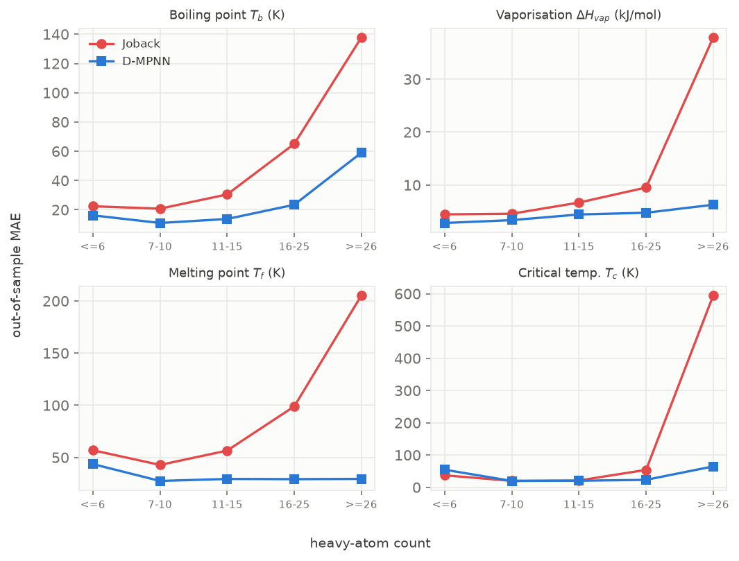
Figure 9. Out-of-sample MAE against heavy-atom count, Joback (red) versus the D-MPNN (blue), on the same held-out folds, for the four properties where Joback covers the size range. Joback's error climbs steeply with molecular size; the graph model's climbs far more slowly (and is flat for melting point and critical temperature).
| property | Joback MAE, smallest / largest bin | D-MPNN MAE, smallest / largest bin |
|---|---|---|
| Boiling point $T_b$ (K) | 22.4 / 138 | 16.2 / 59.0 |
| Vaporisation $\Delta H_{vap}$ (kJ/mol), Joback at 298 K | 4.5 / 37.9 | 2.8 / 6.3 |
| Melting point $T_f$ (K) | 56.9 / 205 | 43.6 / 29.4 |
| Critical temp. $T_c$ (K) | 37.2 / 595 | 54.5 / 64.8 |
Table 6. MAE in the smallest (≤6 heavy atoms) and largest (≥26 heavy atoms) size bins; the largest bin is smallest in count (16 to 66 compounds depending on property), so it is the noisiest, but the trend is monotone across all five bins.
Joback's error grows several-fold from small to large molecules (an order of magnitude for the critical temperature, 37 to 595 K, and about eight-fold for the reference-corrected vaporisation enthalpy), exactly the degradation the paper's premise names, while the D-MPNN's error grows far more slowly, and for melting point and critical temperature is flat, if anything lower on the large molecules than the small ones. It is not flat everywhere: boiling-point and vaporisation-enthalpy D-MPNN error itself rises with size (boiling point 16.2 to 59.0 K across the bins), it simply rises much less steeply than Joback's (22.4 to 138 K), so the accurate statement is "grows far more slowly than Joback's," and "flat" is reserved for the properties ($T_f$, $T_c$) where the table actually shows it. We had expected the degradation to track aromaticity as well as size, since Joback's fitting set is mostly aliphatic; it does not. Splitting each property's Joback error by aromatic-ring membership gives a mixed result (Joback is worse on aromatics for $T_b$, $T_f$ and $\Delta H_{vap}$ but better for $T_c$, $V_c$ and $\Delta G_f$, common aromatics such as benzene and toluene being well inside its fitting set), so the axis that matters is molecular size, not aromaticity.
Where the released family stands against the baselines, after the veto. The release rule of Section 8 makes the correspondence between the tables and the release list checkable. No released model is significantly out-predicted by either baseline; that is the veto working, not an accident. Two released models sit in statistical ties: on critical volume, Joback's nominally lower MAE (0.0148 vs 0.0156 L/mol) is a tie (difference CI $[-0.003, +0.003]$) and the D-MPNN wins on R² (0.988 vs 0.967), so the ranking is Joback ≈ D-MPNN > GBM, a tie at the top rather than a win for either; on the acentric factor the D-MPNN (sum+max) and the GBM are indistinguishable (0.0512 vs 0.0504, CI $[-0.004, +0.006]$). We keep both released, and the line that decides who is served is the veto itself, applied symmetrically: Cheméo serves Joback as the recommended value only where Joback significantly wins (Gibbs energy, critical pressure); on a statistical tie the graph model is served, because it brings what the baseline cannot, the gentler size-degradation of Figure 9 for critical volume plus coverage of the compounds Joback cannot fragment, and applicability to the full corpus for the acentric factor, where Joback offers no estimate at all. The two properties a baseline does significantly beat, Gibbs energy of formation and critical pressure, are exactly the two the veto sends to beta, with Joback served as the recommended value for both. Gibbs energy is the clearest case: on its small, small-molecule-dominated corpus (n = 332, 89% at or below ten heavy atoms) Joback wins every size bin, its extrapolation case is undemonstrated (the large-molecule bins hold 20 and 15 compounds), and it returns to full release only if more large-molecule data shifts the balance. This is a weaker claim than "we replace Joback everywhere," and it is the correct one: the released family is the set of properties where the learned model is at least as good as the incumbent everywhere we can test, and degrades far more gracefully where we cannot.
8.3 On experimental noise as a floor
Several of these properties carry an irreducible experimental scatter that no model can cross. Solubility sits around 0.6 log units on diverse sets [6,8], and melting and fusion data carry polymorphism, purity and decomposition-on-melting [10]. Accuracy is therefore reported next to the relevant reproducibility floor rather than in isolation, and a model whose error approaches that floor is treated as solved for practical purposes.
9. Cross-validation and limitations
The diagnostic sections score a single scaffold split repeated over five seeds. That exposes seed variance but does not pin it down on the smaller sets, where each seed's 10% test is only a few dozen molecules and R² on it is noisy. We therefore re-evaluate every property out-of-sample under repeated scaffold-grouped 10-fold cross-validation: ten folds, three repeats with partition and initialisation both varied, every compound held out exactly once per repeat, each model rebuilt with its own recipe. We lead with MAE, since the pooled cross-validation R² sits on a wider variance denominator than a small held-out sample and is not directly comparable to the single-split R².
Handling acyclic molecules is not optional. About half of most property sets are acyclic, and acyclic molecules share the empty Bemis-Murcko scaffold; binning them as one group forces roughly half the data into a single fold, which is then predicted by a model that has seen no acyclic molecule at all. That manufactures a false failure exactly as a lucky split manufactures a false success. We distribute acyclic molecules across folds (ring scaffolds still never cross a fold) and, as a leakage control, repeat the analysis with Butina similarity-cluster folds so that no near-analogue can straddle train and test.
Cross-validation corrects the release list in both directions (Section 8), and the final list then passes through the Joback veto. The CV confirms seven releases; it flags critical temperature and pressure as flattered by the single split, both falling below the bar out-of-sample; and it rescues Gibbs energy of formation and the acentric factor from the drop list, which single-split seed variance had condemned (rescue here means each is a legitimate model, not that it beats every baseline). Under cross-validation both rescued models are stable across partitions, survive a label-shuffle negative control and a similarity-cluster leakage control, clear the overfit-gap criterion, and reach R² about 0.80 on the ring-containing compounds that make up the single-split test set. The veto and the external benchmark then settle the borderline cases (Section 8): the acentric factor is released; Gibbs energy goes to beta because Joback significantly out-predicts it; critical temperature is promoted on its external CRC validation and its significant win over Joback; critical pressure stays beta, significantly behind Joback. The remaining drops are enthalpy of sublimation (on the R² bar but just past the gap line), dipole moment (a real ceiling for a conformation-dependent property on a 2D graph), and electron affinity, critical compressibility and enthalpy of fusion, close to their data and noise floors.
10. Fitting the final model on all the data
Cross-validation estimates how well the recipe generalises, and that estimate is what Section 8 reports. Once we have it, the held-out test set has done its job. For the final model, we want that data back in the training set: a model fit on all the data is at least as good as one fit on nine tenths of it, and cross-validation has already measured the error, so there is nothing left to compute on a held-out split. So we fit each released property one last time on the full dataset.
That raises a question that only appears once the test set is gone: with no held-out data, when do we stop training? Early stopping needs a validation signal, and on the smaller sets a ten-percent slice is only a few dozen molecules, its loss is noisy, and the epoch it stops at swings enough to sometimes return an under-trained model. We instead read the stopping epoch off the convergence curve itself (Figure 10): run the training once to the full budget, average the validation-loss curve over several seeds to smooth it, and stop a few epochs into the plateau (the first epoch within one percent of the minimum, plus three).
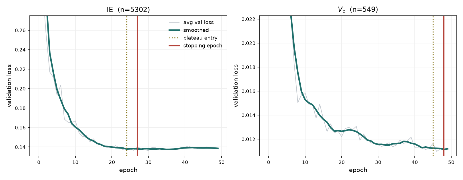
Figure 10. Validation loss against epoch for a large property (ionisation energy) and a small one (critical volume). Dotted line: plateau entry, the first epoch within 1% of the smoothed minimum. Solid line: the chosen stopping epoch, three epochs later.
The plateau falls at a different epoch for each property, and in the counterintuitive direction: the large sets converge early (boiling point by about epoch 20) and the small sets later (critical volume about 45), because a smaller set takes fewer gradient steps per epoch. A single global budget would under-train the small models and over-train the large ones, so the stopping epoch is set per property: $T_b$ 26, IE 27, $T_f$ 35, $\log_{10}S$ 36, $\Delta H_{vap}$ 38, $\Delta H_f$ 42, $V_c$ 48, $\omega$ 30 and $\Delta G_f$ 45. The rule is mechanical, including its fallbacks, so it can be reproduced exactly. The primary rule is the first epoch within 1% of the smoothed minimum, plus three. When the averaged curve is too noisy for any epoch to fall within 1% of the minimum, the tolerance is dropped and we take the epoch of the smoothed minimum itself, plus three. For the two data-starved beta models whose loss dips, bounces and re-converges (critical temperature and pressure), the minimum is taken over the re-converged region rather than the pre-bounce dip. No hand-tuning enters beyond these three cases, each stated. This is safe because the averaged validation loss does not rise materially before the fifty-epoch budget ends: for every released property its minimum-to-epoch-50 increase is a few percent, well inside the plateau, so any stop within the plateau gives essentially the same model and erring a few epochs late costs nothing. A remaining gap is that the fixed-epoch heuristic is validated only indirectly, through the flatness of the plateau; a direct check would compare the fixed-epoch model to the early-stopped model on a genuinely held-out split for a few properties, to confirm the fixed epoch neither over- nor under-trains relative to early stopping. The final model for each property is thus trained on every available compound, with the stopping epoch taken from the convergence curve rather than from a held-out signal that, by design, no longer exists.
10.1 Limitations of the deployed models: applicability domain and uncertainty
Two limitations matter most for a tool served at a public endpoint. First, the shipped models return a bare point prediction with no applicability-domain flag and no per-prediction uncertainty. This is the practically important gap precisely because the paper stakes the family's value on size-extrapolation: the error grows where the molecule is large or the scaffold rare (Sections 6, 8.2), and two results make it concrete. The sharper one is the released critical-temperature model: the 1.7% of its compounds that are bare elements or near-atomic species carry a mean error of about 450 K (Section 8.2), so a user querying $T_c$ for, say, mercury today receives a confidently wrong number with no warning, where Joback at least declines. The broader one is the enthalpy-of-formation external tail (about 9% of a broad external set beyond 100 kJ/mol, Section 8.1). Both are exactly the out-of-support regime a user cannot currently see they are in: a user given "-250 kJ/mol" has no signal whether the compound sits in the dense core of the training distribution or far outside it. A lightweight remedy we intend to add to the served models is a domain flag, a distance to the training set in the learned or a fingerprint space, or an ensemble-variance estimate from the five-seed fleet already trained (Appendix A.3), returned alongside the value so an extrapolating prediction is marked as such; nearest-neighbour and conformal-style intervals are the natural next step. Second, and relatedly, the fixed-epoch serving heuristic (above) is validated only indirectly, through plateau flatness. Neither limitation changes the released numbers, but both bound how the deployed tool should be read, and the applicability-domain flag is the single change that would most improve it in practice.
A property-prediction tool built on these models is available free of charge at https://www.chemeo.com/predict.
Appendix A. Complete specification for reproduction
This appendix gives every element needed to reproduce the models, in framework-neutral terms. We use Chemprop v2.2.4 [2], but each piece below is standard and can be built in any graph-learning toolkit.
A.1 Atom and bond features
Each atom is a 72-dimensional vector, each bond a 14-dimensional vector, both one-hot with an extra bucket for values outside the listed set (marked "+ unknown"), plus two scalar atom features.
Atom features (72):
| block | encodes | size |
|---|---|---|
| atomic number | Z in 1 to 36, and 53 (iodine), + unknown | 38 |
| degree | 0 to 5, + unknown | 7 |
| formal charge | -1, -2, +1, +2, 0, + unknown | 6 |
| chiral tag | 4 RDKit tags, + unknown | 5 |
| hydrogen count | 0 to 4, + unknown | 6 |
| hybridization | s, sp, sp2, sp2d, sp3, sp3d, sp3d2, + unknown | 8 |
| aromaticity | boolean | 1 |
| mass | atomic mass / 100 | 1 |
Table 7. Atom feature blocks and their dimensions (72 total).
Bond features (14):
| block | encodes | size |
|---|---|---|
| null bond | whether the bond is absent | 1 |
| bond type | single, double, triple, aromatic | 4 |
| conjugated | boolean | 1 |
| in ring | boolean | 1 |
| stereo | 6 RDKit stereo classes, + unknown | 7 |
Table 8. Bond feature blocks and their dimensions (14 total).
A.2 Message-passing equations
The network is the directed MPNN of Yang et al. [1]. Write $\mathbf{x}_v$ for the atom features of atom $v$, $\mathbf{e}_{vw}$ for the bond features of the directed bond $v \to w$, $[\,\cdot\,;\,\cdot\,]$ for concatenation, and $\mathcal{N}(v)$ for the neighbours of $v$. All weight matrices have no bias, the activation is $\mathrm{ReLU}$, the hidden width is $h = 300$, and the depth is $T = 3$.
Edge initialisation, with $\mathbf{W}_i \in \mathbb{R}^{300 \times 86}$:
Message passing, for $t = 1, \dots, T$, with $\mathbf{W}_h \in \mathbb{R}^{300 \times 300}$. The message into the directed bond $v \to w$ sums the incoming bond states at $v$ but excludes the reverse bond $w \to v$, which is what makes it directed:
Atom representation, with $\mathbf{W}_o \in \mathbb{R}^{300 \times 372}$:
Molecule readout, the choice this paper is about, with $\mathrm{AGG}$ one of mean, sum, max, or a concatenation of these:
Prediction, where $s(\mathbf{d})$ is the fitted descriptor transform (A.4, only for the +2D models, concatenated when used) and $\sigma_y$ is the training-set target standardisation:
The head $\mathrm{FFN}$ is one hidden layer of width 300 with $\mathrm{ReLU}$, then a linear map to the scalar output. With a mean readout this is about 318,000 trainable weights: about 228,000 in $\mathbf{W}_i$, $\mathbf{W}_h$, $\mathbf{W}_o$, about 91,000 in the head, none in the readout.
A.3 Architecture and training hyperparameters
| item | value |
|---|---|
| hidden width | 300 |
| message-passing depth | 3 |
| activation | ReLU |
| message-passing bias | none |
| dropout | 0 |
| batch normalisation | none |
| readout | per property, listed in Appendix A.9 (mean, sum+max, or mean+sum+max) |
| head | 1 hidden layer, width 300, ReLU |
| target scaling | standardise (mean 0, sd 1) on the training split; predictions mapped back to physical units |
| loss | mean squared error, in scaled space |
| optimiser | Adam |
| learning-rate schedule | linear warmup over 2 epochs from 1e-4 to 1e-3, then decay to 1e-4 |
| batch size | 64 |
| max epochs | 50 |
| early stopping | on validation loss, patience 10, best-validation weights restored |
| seeds | 42 to 46, five independent repeats for the diagnostics; each seed sets its own scaffold split and training run |
| release evaluation | repeated scaffold 10-fold cross-validation (three repeats, every compound held out once); the reported MAE/R² are these out-of-sample numbers |
| final model | refit on the full dataset at a fixed per-property epoch, no early stopping (Section 10); because it trains on more data than any cross-validation fold, the reported numbers are a conservative estimate of its accuracy |
Table 9. Architecture and training hyperparameters, shared by every property model.
A.4 Descriptor augmentation (the +2D models)
The six +2D models concatenate 15 conformer-free RDKit descriptors to the molecule vector $\mathbf{h}_G$, before the head. None needs a 3D conformer.
Symmetry: fraction of atoms with a unique canonical rank, and the fraction that are symmetry-equivalent to another atom (both from Chem.CanonicalRankAtoms(breakTies=False)).
Shape: fraction of atoms in aromatic rings.
Flexibility: rotatable-bond count, rotatable-bond fraction, ring count, count of ring-shared bonds, and fraction of sp3 carbons.
Interaction: H-bond donors, H-bond acceptors, TPSA, and the sum of absolute formal charges.
Size: molecular weight, heavy-atom count, and total atom count.
Scaling, fitted on the training split only: missing values are imputed to the training median; the strictly-positive heavy-tailed columns (rotatable-bond count, ring count, ring-shared-bond count, TPSA, molecular weight, heavy-atom count, atom count) are log1p-transformed; then a RobustScaler (median-centred, scaled by the interquartile range) is applied. A plain StandardScaler is deliberately avoided, because these descriptors are far from normally distributed.
A.5 Readout variants: mean versus sum+max
The readout is the choice this paper turns on, so we give each variant explicitly. Write $V$ for the atoms of molecule $G$, $\mathbf{h}_v \in \mathbb{R}^{d}$ for the per-atom embedding after message passing ($d = 300$; A.2), $[\,\cdot\,;\,\cdot\,]$ for concatenation along the feature axis, and subscript $j$ for a feature index. The four readouts compared in Section 5 are:
Two differences carry the whole result. The mean divides the summed contributions by the atom count $|V|$, so it is size-invariant: two molecules with the same average atom map to the same vector regardless of size. The sum does not divide, so the molecule vector grows with the molecule and the readout is extensive in the graph sense (graph-extensive; the network's output scales with atom count, distinct from whether the target property is thermodynamically extensive, Section 5). The max keeps, per feature, the single most extreme atom, the signal a lone functional group carries and the average washes out.
The head consumes $\mathbf{h}_G$, so its input width is $k\,d + w$, where $k \in \lbrace 1, 2, 3\rbrace $ is the number of concatenated pooling channels and $w$ is the descriptor width (15 for the +2D models, 0 otherwise). Only this width changes across readouts; the message-passing weights are identical, so comparing readouts is the same graph encoder with a wider or narrower head, not a different network. In practice each pooling is a single batched segment-reduce (sum, mean, or amax) over the atoms grouped by molecule, so the extra channels add a few lines and no learned weights in the encoder.
A.6 Data pipeline
Experimental values are pulled from the Cheméo API. For each compound, only measured values are kept, the structure is parsed from the InChI first with a SMILES fallback, and bare elements with no heavy atom are dropped. Values are deduplicated by canonical SMILES, keeping the median when several measurements exist, and filtered to a coarse physical range per property. The stored conditions are the standard ones for each property (normal boiling and melting points at 1 atm; formation and Gibbs energies as standard gas-phase values at 298.15 K; vaporisation enthalpy at 298.15 K (confirmed by the external check in Section 8.1, where the model matches the 298 K CRC column and not the boiling-point column); aqueous solubility as the value tabulated by Cheméo; critical constants are condition-free), and where the database aggregates measurements at differing conditions the median absorbs the scatter, which the per-compound spread column records.
Per-property counts, the fraction of compounds with more than one measurement (a coarse redundancy indicator), and the plausibility-range filter:
| property | unit | n | multi-measurement | range filter kept |
|---|---|---|---|---|
| $T_b$ | K | 4948 | 47% | 50 to 2000 |
| $T_f$ | K | 4433 | 44% | 30 to 2000 |
| $T_c$ | K | 1054 | 46% | 50 to 2500 |
| $P_c$ | kPa | 917 | 40% | 100 to 30000 |
| $V_c$ | L/mol | 549 | 25% | 0.05 to 5 |
| $Z_c$ | - | 511 | 0% | 0.1 to 0.5 |
| $\omega$ | - | 599 | 0% | -0.5 to 1.5 |
| $\Delta H_f$ | kJ/mol | 2337 | 31% | -8000 to 2000 |
| $\Delta G_f$ | kJ/mol | 332 | 0% | -5000 to 1000 |
| $\Delta H_{vap}$ | kJ/mol | 2496 | 45% | 1 to 500 |
| $\Delta H_{sub}$ | kJ/mol | 1343 | 47% | 1 to 500 |
| $\Delta H_{fus}$ | kJ/mol | 525 | 14% | 0.1 to 200 |
| $\log_{10}S$ | log₁₀(mol/L) | 2104 | 50% | -15 to 3 |
| IE | eV | 5302 | 51% | 3 to 30 |
| EA | eV | 637 | 49% | -2 to 6 |
| $\mu$ | Debye | 301 | 0% | 0 to 12 |
Table 10. Per-property compound counts, the fraction of compounds with more than one measurement, and the plausibility range each property is filtered to.
The split is a balanced Bemis-Murcko scaffold split into 0.8 / 0.1 / 0.1 train / validation / test. The diagnostic experiments in Sections 4 to 7 use one such split frozen at seed 42; Section 8 evaluates every property out-of-sample by repeated scaffold cross-validation (Section 9), and the final model is a full-data refit (Section 10).
A.7 Diagnostic procedures
The GBM sanity baseline is a scikit-learn HistGradientBoostingRegressor (300 iterations, random state 0) on 12 RDKit descriptors: molecular weight, MolLogP, TPSA, H-bond acceptors, H-bond donors, rotatable bonds, ring count, fraction sp3, valence-electron count, aromatic-ring count, heavy-atom count, and saturated-ring count.
It is trained and evaluated on the same split as the graph model.
The mean-collapse check is $\mathrm{std}(\hat{y}) / \mathrm{std}(y)$ on the test set, and the model RMSE against the RMSE of predicting the training mean; for a single-target regression,
Target transforms, applied outside the model and inverted at prediction: identity (default), log10 for strictly-positive heavy-tailed targets, and per-heavy-atom (divide by heavy-atom count, multiply back) for extensive targets.
A.8 Software versions
python 3.11, chemprop 2.2.4, RDKit 2026.03, PyTorch 2.12 (CPU), PyTorch Lightning 2.6, scikit-learn 1.9, numpy 2.4, thermo 0.6.0 (Joback and the CRC critical-property tables), chemicals 1.5.2.
The specification in this appendix is sufficient to reproduce the models.
A.9 Full property roster and release decisions
All sixteen properties in one place, so the release rule can be audited row by row. The rule has two parts (Section 8): the statistical bar (out-of-sample R² ≥ 0.70 with train-test gap ≤ 0.20 under repeated scaffold CV, or state-of-the-art accuracy on a shared external benchmark) and the Joback veto (the incumbent must not significantly out-predict the model, by the scaffold-cluster paired bootstrap of Section 8.2). Numbers are the three-repeat scaffold-CV aggregate on the per-repeat (single-model) basis, the same evaluation as Section 8 and the Section 8.2 head-to-head.
| property | symbol | n | readout | 2D | CV MAE | CV RMSE | CV R² | released |
|---|---|---|---|---|---|---|---|---|
| Ionisation energy | IE | 5302 | sum+max | - | 0.344 | 0.608 | 0.795 | yes |
| Normal boiling point | $T_b$ | 4948 | mean+sum+max | - | 13.5 | 30.2 | 0.879 | yes |
| Normal melting point | $T_f$ | 4433 | mean+sum+max | yes | 30.8 | 56.3 | 0.744 | yes |
| Enthalpy of vaporisation | $\Delta H_{vap}$ | 2496 | sum+max | yes | 3.69 | 6.75 | 0.949 | yes |
| Enthalpy of formation | $\Delta H_f$ | 2337 | sum+max | - | 35.5 | 64.5 | 0.974 | yes |
| Aqueous solubility | $\log_{10}S$ | 2104 | mean+sum+max | - | 0.560 | 0.771 | 0.877 | yes |
| Enthalpy of sublimation | $\Delta H_{sub}$ | 1343 | mean+sum+max | - | 12.9 | 20.0 | 0.665 | no |
| Critical temperature | $T_c$ | 1054 | sum+max | yes | 33.1 | 84.8 | 0.657 | yes‡ |
| Critical pressure | $P_c$ | 917 | mean+sum+max | yes | 487 | 1390 | 0.585 | beta† |
| Electron affinity | EA | 637 | mean+sum+max | yes | 0.456 | 0.670 | 0.411 | no |
| Acentric factor | $\omega$ | 599 | sum+max | - | 0.0512 | 0.0795 | 0.781 | yes |
| Critical volume | $V_c$ | 549 | mean+sum+max | yes | 0.0156 | 0.0242 | 0.988 | yes |
| Enthalpy of fusion | $\Delta H_{fus}$ | 525 | sum+max | - | 11.8 | 18.6 | 0.431 | no |
| Critical compressibility | $Z_c$ | 511 | mean+sum+max | yes | 0.0129 | 0.0219 | 0.218 | no |
| Gibbs energy of formation | $\Delta G_f$ | 332 | sum+max | - | 42.2 | 97.3 | 0.840 | beta† |
| Dipole moment | $\mu$ | 301 | mean+max | yes | 0.385 | 0.559 | 0.678 | no |
Table 11. All sixteen properties with their readout, cross-validation numbers, and release decision. Numbers are the three-repeat scaffold-CV aggregate on the per-repeat (single-model) basis.
The five fully held-back properties and the reason each misses: enthalpy of sublimation (R² 0.67, just under the bar with a gap fractionally over 0.20, and no external set to enter by); electron affinity (0.41), enthalpy of fusion (0.43) and critical compressibility (0.22), all near their data or noise floors; and dipole moment (0.68, a conformation-dependent property a 2D graph cannot fully resolve). The melting-point / sublimation pair sits either side of the bar: $T_f$ at R² 0.744 clears it, $\Delta H_{sub}$ at 0.665 does not.
†Beta under the Joback veto: each clears or approaches the statistical bar, but Joback significantly out-predicts it on the same held-out folds ($\Delta G_f$ 22.4 vs 42.2 kJ/mol; $P_c$ 300 vs 487 kPa), so Cheméo serves the Joback estimate as the recommended value and the graph model as beta (Sections 8 and 8.2).
‡Released under the external arm of the rule: below the scaffold-CV bar (0.657, the conservative number, shown here), but externally validated at the state of the art on the held-out CRC set (R² 0.916, Section 8.1) and a significant win over Joback (Section 8.2).
References
[1] K. Yang, K. Swanson, W. Jin, C. Coley, P. Eiden, H. Gao, A. Guzman-Perez, T. Hopper, B. Kelley, M. Mathea, et al. Analyzing Learned Molecular Representations for Property Prediction. Journal of Chemical Information and Modeling, 59(8):3370-3388, 2019. https://doi.org/10.1021/acs.jcim.9b00237
[2] E. Heid, K. P. Greenman, Y. Chung, S.-C. Li, D. E. Graff, F. H. Vermeire, H. Wu, W. H. Green, C. J. McGill. Chemprop: A Machine Learning Package for Chemical Property Prediction. Journal of Chemical Information and Modeling, 64(1):9-17, 2023. https://doi.org/10.1021/acs.jcim.3c01250
[3] F. T. Mtetwa, N. F. Giles, W. V. Wilding, T. A. Knotts IV. Prioritizing Data Quality in Machine Learning for Thermophysical Property Prediction: A Case Study on Normal Boiling Points of Organic Compounds. ACS Omega, 10(42):49794-49804, 2025. https://doi.org/10.1021/acsomega.5c05503
[4] A. N. Marimuthu, B. A. McGuire. Machine Learning Pipeline for Molecular Property Prediction Using ChemXploreML. Journal of Chemical Information and Modeling, 2025. https://doi.org/10.1021/acs.jcim.5c00516 (preprint: arXiv:2505.08688)
[5] R. Bounaceur, F. Paes, R. Privat, J.-N. Jaubert. AI-powered prediction of critical properties and boiling points: a hybrid ensemble learning and QSPR approach. Journal of Cheminformatics, 2025. https://doi.org/10.1186/s13321-025-01062-9
[6] A. Llinàs, R. C. Glen, J. M. Goodman. Solubility Challenge: Can You Predict Solubilities of 32 Molecules Using a Database of 100 Reliable Measurements? Journal of Chemical Information and Modeling, 48(7):1289-1303, 2008. https://doi.org/10.1021/ci800058v
[7] A. Llinàs, A. Avdeef. Solubility Challenge Revisited after Ten Years, with Multilab Shake-Flask Data, Using Tight (SD ~ 0.17 log) and Loose (SD ~ 0.62 log) Test Sets. Journal of Chemical Information and Modeling, 59(6):3036-3040, 2019. https://doi.org/10.1021/acs.jcim.9b00345
[8] P. Llompart, C. Minoletti, S. Baybekov, D. Horvath, G. Marcou, A. Varnek. Will we ever be able to accurately predict solubility? Scientific Data, 11, 2024. https://doi.org/10.1038/s41597-024-03105-6
[9] S. Boobier, A. Osbourn, J. B. O. Mitchell. Can human experts predict solubility better than computers? Journal of Cheminformatics, 9:63, 2017. https://doi.org/10.1186/s13321-017-0250-y
[10] L. E. Austermeier, K. Voigt, A. Böhme, N. Ulrich. Prediction of Melting Points of Chemicals with a Data Augmentation-Based Neural Network Approach. ACS Omega, 10(23):24296-24306, 2025. https://doi.org/10.1021/acsomega.5c00205
[11] M. Karthikeyan, R. C. Glen, A. Bender. General Melting Point Prediction Based on a Diverse Compound Data Set and Artificial Neural Networks. Journal of Chemical Information and Modeling, 45(3):581-590, 2005. https://doi.org/10.1021/ci0500132
[12] H. Brykczynski, J. Seilert, E. Flöter. Prediction of Melting Point Temperatures and Enthalpies of Fusion for Pure Wax Esters Using a Group Contribution Model. Crystal Growth & Design, 25(16):6697-6709, 2025. https://doi.org/10.1021/acs.cgd.5c00684
[13] R. J. C. Brown, R. F. C. Brown. Melting Point and Molecular Symmetry. Journal of Chemical Education, 77(6):724, 2000. https://doi.org/10.1021/ed077p724
[14] K. G. Joback, R. C. Reid. Estimation of Pure-Component Properties from Group-Contributions. Chemical Engineering Communications, 57(1-6):233-243, 1987. https://doi.org/10.1080/00986448708960487
[15] J. Marrero, R. Gani. Group-contribution based estimation of pure component properties. Fluid Phase Equilibria, 183-184:183-208, 2001. https://doi.org/10.1016/S0378-3812(01)00431-9
[16] G. Landrum, P. Tosco, B. Kelley, et al. RDKit: Open-source cheminformatics. 2026. https://www.rdkit.org, https://doi.org/10.5281/zenodo.20446949
[17] L. d'Anterroches. Cheméo: Open Database of Chemical Properties. 2026. https://www.chemeo.com
[18] K. Xu, W. Hu, J. Leskovec, S. Jegelka. How Powerful are Graph Neural Networks? International Conference on Learning Representations (ICLR), 2019. https://arxiv.org/abs/1810.00826
[19] G. Corso, L. Cavalleri, D. Beaini, P. Liò, P. Veličković. Principal Neighbourhood Aggregation for Graph Nets. Advances in Neural Information Processing Systems (NeurIPS), 33:13260-13271, 2020. https://arxiv.org/abs/2004.05718
[20] C. Bell, and Contributors. chemicals: Chemical properties component of Chemical Engineering Design Library (ChEDL). 2016-2024. https://github.com/CalebBell/chemicals